The Point Rainfall product aims to deliver probabilities for point measurements of rainfall (within a forecast model gridbox). “ecPoint” is the name given to the post-processing philosophy and software package.

To understand the concept, let us first consider the radar-derived rainfall totals shown on the example in Figure 1. We assume that these are accurate, meaning that they indicate what would have been measured locally by rain gauges. Then consider the ECMWF ensemble (ENS) gridbox highlighted. Within this box, whilst the gridbox average rainfall total is about 17mm, the minimum and maximum rainfall amounts are about 2mm and 60mm respectively. This implies a lot of sub-grid variability. A completely accurate ensemble member forecast would predict 17mm. But clearly this of itself would give the user no idea that locally there was much more (and indeed much less) than this amount. And to cause flash floods, as were observed, probably a 17mm total, locally, would not have been enough. The point rainfall approach aims to estimate the range of totals likely within the gridbox, and indeed it delivers probabilities for different point values within that gridbox (albeit without saying where the largest and smallest amounts are likely to be).

Figure 1.
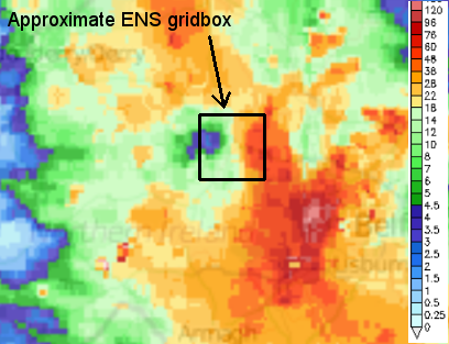
Radar-derived rainfall totals over part of Northern Ireland for the 12h period ending 00UTC 29 July 2018. Scale is in mm. Flash floods occurred in some locations. Figure based on data from netweather.tv

4 main aspects of ecPoint can be highlight:

• The new product is a post-processed product from the ECMWF ensemble system, which calibrates ensemble fields, including the control run.
• It delivers probabilistic forecasts of rainfall totals for points – i.e. that would be measured by a rain gauge randomly located within a model gridbox (hence the word ‘point’)
• By way of comparison, the raw ensemble delivers probabilities for gridbox-average rainfall (in the current ensemble that means ~18x18km boxes, up to day 10)
• The term rainfall here means all precipitation types: rain, rain plus snow, snow etc., always converted into mm of rain equivalent.

There are two reasons why point rainfall and ensemble rainfall distributions commonly differ:

• Sub-grid variability – Figure 1 shows an example of large sub-grid variability – which itself varies according to the weather-type in a gridbox.
• Model biases, on the gridscale, also intrinsic to the weather type in a gridbox.

“Weather type” here refers to specific weather conditions inside a gridbox – e.g. “mainly convective precipitation with strong mid-level winds, …”. In practice, ecPoint post-processing creates, on the basis of the calibration results (see below), an “ensemble of ensembles”, that is 100 new point rainfall realisations for each ensemble member, and so comprises, at one intermediate stage in the computations, 5100 equi-probable values of point rainfall totals within each ensemble gridbox. However, prior to saving, the values for each gridbox are sorted, and distilled down into 99 percentile fields (1,2,..99). As a set these percentile fields constitute the Point Rainfall product.

Figure 2 shows examples of cumulative distribution functions (CDFs) for different sites on two different occasions, for the full ECMWF ensemble, illustrating the two types of adjustment that ecPoint makes, bias correction and the addition of sub-grid variability. These adjustments are most in evidence on the first plot, whilst the second plot shows also that the point rainfall and raw model gridscale distributions may sometimes be quite similar.

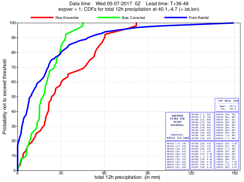
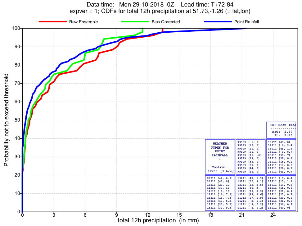
Figure 2.
Two CDF examples comparing raw gridscale (red), post-processed bias-corrected gridscale (green), and post-processed point rainfall (blue). The first plot is for a site in Spain in summer at day 2. The second plot is for a southern England site in autumn, at day 4. Note that for each case the areas to the left of the green and blue curves, that represent the mean gridbox rainfall over the ENS, should be the same. Note also that these plots show forecasts for 12h rainfall, whilst in MISTRAL we create forecasts for 6h periods.

Outputformats
We currently make available overlapping 6h periods up to day 10, namely T+0-T+6, T+3-T+9,..T+234-T+240

Calibration
As with any post-processing system ecPoint has to be calibrated. For this it uses short-range control run forecasts of 6h rainfall covering one year (the “training period”), which are individually compared with rainfall observations, for the same times, within the respective gridboxes. The full procedure is not described here but involves segregation according to gridbox-weather-types, which each have different sub-grid variability structures and/or different bias corrections associated. The 6h point rainfall system introduced by ECMWF for MISTRAL incorporated 245 such types. The type definitions are currently based on the following parameters: convective rainfall fraction, total 6h precipitation forecast, solar radiation, local solar time, standard deviation of the filtered orography, 700hPa wind speed and CAPE

Some Uses of Point Rainfall
By giving, for example, non-zero probabilities for very large totals that had a zero probability in the raw ensemble output, the Point Rainfall can provide a useful new pointer to when flash floods are possible locally. Likewise, if one wants a better idea of how likely it is that a given period remains dry, the point rainfall can usually provide better guidance; indeed, in convective (showery) situations the point rainfall probabilities for dry should be much better. And where a certain criterion has to be met as the basis for a warning or alert, which might not always be a large total, again the point rainfall should overall provide customers with better guidance than the raw ensemble.

More information: https://confluence.ecmwf.int/display/FUG/Point+Rainfall

COSMO-2I POST-PROCESSING

The product from post-processing COSMO-2I-EPS is called Cosmo-2Ipp and is related to the computation of the agreement scale S between the different ensemble members, according to the following procedure, more thoroughly described in Dey et. al (2016a, 2016b) and Blake et al. (2018):

1. At grid point P of the model, the difference in precipitation between all the ensemble members is considered; i.e. their similarity is assessed. This comparison process is based on examining pairs of ensemble members separately, using all possible combinations. For the COSMO-2I-EPS, which has 20 members, this means 190 separate comparisons.
2. If the forecasts are found to be quite similar (that is if the differences are below a certain threshold), then the agreement scale at point P is the grid scale of the model itself. If the fields are not that similar, then a square neighbourhood size = 3 x 3 grid points, centred upon the point P, is considered.
3. Again the spatial precipitation averages, considering the 3×3 grid point sets for all ensemble members, are compared and their similarity is assessed.
4. If, this time, the forecasts are found to be quite similar, then the agreement scale is set to 3×3. If the fields are not similar enough, then the scale is increased again, to give a 5×5 grid‐point neighbourhood.
5. Until the agreement scale has been set, the code will repeat steps similar to 3) and 4), incrementing the neighbourhood size each time. At some pre-defined level computations will stop even if agreement has not been reached – this is for computational efficiency reasons.
6. Then the agreement scale (i.e. a neighbourhood size) defines which points’ values around P will be used to deliver the probability distribution for rainfall at P. For example, if the agreement scale is 3×3, we use 20*3*3 = 180 different values from the 20 ensemble members. These values, ranked, define the rainfall CDF for point P, and we conclude by computing from this CDF percentiles 1-99 for precipitation at point P (irrespective of how many different values contributed to its CDF). These percentiles are stored.
7. The previous steps are repeated at all grid points

The percentiles computed following this procedure are then combined with those generated by ecPoint-rainfall, to deliver a blended product for short-to-medium range ensemble forecasts.

BLENDING COSMO-ECPOINT

Cosmo-2Ipp-ecPoint is a set of probabilistic 6-h precipitation forecast products, for Italy and surrounding countries, up to day 10. It consists of 2 different types of product, depending on the lead time of the forecast:

• From 0 to 48h: blending of ecPoint rainfall & COSMO-2I-EPS post-processed, with different weights applied in that blending, depending on the lead time. More weight is given to COSMO-2I-EPS at shorter lead times, tapering to about zero at 48h. The horizontal resolution of the product is 2.2 km and time resolution is 3-hourly.
• From 48h to 240h (day 10): Only ecPoint rainfall is available, at 18 km horizontal resolution. The time resolution is 3-hourly from 48 to 144h and 6-hourly from 144h to 240h.

The “tapered blending” strategy means that through all the lead times, and indeed across the 48h “barrier”, the forecast evolution should look relatively smooth to users, with more detail apparent at the shortest leads. The intention was to create an accurate, useful, seamless forecast.

The final products are created twice a day, blending firstly ecPoint from the 12UTC ECMWF ensemble with the 21UTC COSMO-2I-EPS outputs, and then when the 00UTC ECMWF ensemble data becomes available that is blended with the same 21UTC COSMO data, to deliver an “update”. Two different products are produced:

1. Probabilities of exceeding specific 6-h total precipitation thresholds: the available thresholds in the catalogue are: 5, 10, 20 and 50 mm.
2. Percentiles: the available percentiles are: 1, 10, 25, 50, 75 and 99.

EcPoint is specifically designed to improve the reliability and discrimination ability of the forecast. In verification it shows some particularly good results for large totals. Furthermore, by combining with the COSMO ensemble output we improve the forecasts even more. And in certain situations, we can give increased specificity regarding where the most extreme totals are most likely to occur.

References:
Blake, B.T., Carley, J.R., Alcott, T.I., Jankov, I., Pyle, M.E., Perfater, S.E. and Albright B (2018), An Adaptive Approach for the Calculation of Ensemble Gridpoint Probabilities. Wea. Forecasting, 33: 1063–1080. https://doi.org/10.1175/WAF-D-18-0035.1

Dey, S.R.A., Roberts, N.M., Plant, R.S. and Migliorini, S. (2016a), A new method for the characterization and verification of local spatial predictability for convective‐scale ensembles. Q.J.R. Meteorol. Soc., 142: 1982-1996. doi:10.1002/qj.2792

Dey, S.R.A., Plant, R.S., Roberts, N.M. and Migliorini, S. (2016b), Assessing spatial precipitation uncertainties in a convective‐scale ensemble. Q.J.R. Meteorol. Soc., 142: 2935-2948. doi:10.1002/qj.289